INGARCH and GLARMA Models for Count Time Series in Fable Framework • fableCount

The fableCount R package aims to offer counting time series models for users of the fable framework. These models work within the fable framework, which provides the tools to evaluate, visualize, and combine models in a workflow consistent with the tidyverse.

Installation

You can install the stable version from CRAN:

install.packages("fableCount")

You can install the development version from GitHub

# requires("devtools")
remotes::install_github("Gustavo039/fableCount")

Count Time Series

A count time series is a sequence of observations that record the number of events occurring at discrete time intervals. These events can be anything that can be counted, such as the number of daily sales, the number of calls received per hour, or the number of cases of a disease per week.

INGARCH and GLARMA usage

The package has 2 main functions.

INGARCH - (Integer Generalized Autoregressive Conditional Heteroskedasticity)
GLARMA - (Generalized Linear Autoregressive Moving Averages)

The usage of the model functions follows the fable and fabletools pattern

dataset |>
  fabletools::model(
    model_name1 = INGARCH(response_variable ~ pq(AR_oder, MA_order)),
    model_name2 = GLARMA(response_variable ~ pq(AR_oder, MA_order))
    )

If the pq() is ommited, the automatic parameter selection algorithm is triggered. Such algorithms are based on searching for the model that presents the lowest AIC or BIC

Example - Influeza in Germany

The following dataset was taken from the tscount package and gives the weekly number of reported influenza cases in the state of North Rhine-Westphalia (Germany) from January 2001 to May 2013.

(The cleaned tsibble object can be obtained via fableCount::influenza_rhine)

influenza_rhine |>
  autoplot() +
  labs(title = "Influenza Cases in Rhine-Westphalia, Germany",
       y="Number of Cases") +
  theme_minimal()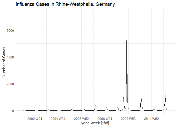

For models estimation, the automatic parameter selection method was used

model_influenza = influenza_rhine |>
  model(ing = INGARCH(cases),
        gla = GLARMA(cases, method = 'NR'))

The estimated models were:

INGARCH

model_influenza |> 
  select(ing) |>
  report()
#> Series: cases 
#> Model: INGARCH(2, 0) 
#> 
#> poisson INGARCH(2, 0) w/ identity link
#> # A tibble: 2 × 4
#>   statistic `(Intercept)`  beta_1   beta_2
#>   <chr>             <dbl>   <dbl>    <dbl>
#> 1 Estimate         0.202  0.986   1.04e-10
#> 2 Std.Error        0.0245 0.00864 7.29e- 3
#> 
#> log likelihood=-10521.42
#> AIC=21048.83
#> BIC=21062.24
#> QIC=21049.86

GLARMA

model_influenza |> 
  select(gla) |>
  report()
#> Series: cases 
#> Model: GLARMA(1, 0) 
#> 
#> Poisson GLARMA(1, 0)
#> # A tibble: 2 × 3
#>   statistic intercept      ar_1
#>   <chr>         <dbl>     <dbl>
#> 1 estimate    3.92    0.0154   
#> 2 std_error   0.00608 0.0000291
#> 
#> log likelihood=-59377
#> AIC=118758

With the models already estimated, it is possible to draw a prediction interval

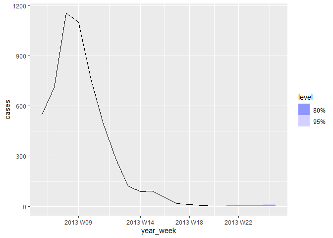
INGARCH forecast

model_influenza |> 
  dplyr::select(ing) |>
  forecast(h = 5) |>
  autoplot(influenza_rhine |>
             dplyr::filter(year_week > tsibble::make_yearweek(2013, 5) )
           )

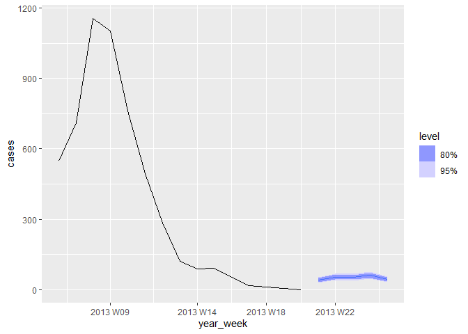
GLARMA forecast

model_influenza |> 
  dplyr::select(gla) |>
  forecast(h = 5) |>
  autoplot(influenza_rhine |>
             dplyr::filter(year_week > tsibble::make_yearweek(2013, 5) )
           )

Learning to forecast with fable

The forecasting principles and practices online textbook provides an introduction to time series forecasting using fable: https://otexts.com/fpp3/